Economic Voting

Focusing on Presidential elections, Achen & Bartels (2017) demonstrate that short-term economic growth is a strong predictor of the popular vote margin of the President’s party. They argue that the growth in real disposable income (RDI) per capita in the 2nd and 3rd quarter of the Presidential election year is a better predictor than cumulative growth.

Keeping this in mind, I hypothesize that short-term changes in the state of the economy in the leadup to Congressional elections are strong predictors of how well the incumbent President’s party performs. Similar to Achen & Bartels (2017), I focus on the state of economy in the 2nd and 3rd quarter of the election year (Q6 and Q7). Focusing on Congressional elections between 1948 and 2020, I measure the performance of the President’s party by calculating the President’s party’s two-party vote share. As seen in Table 1, the independent variables in Models (1) ~ (6) are the RDI growth between Q6 and Q7, gross domestic product (GDP) growth between Q6 and Q7, unemployment in Q7, and whether the election is a midterm election. I included a dummy variable for midterms because the President’s party tends to lose seats in midterm elections (Campbell, 2018, p. 1).

What’s wrong with these models?: Multicollinearity & Outlier

As seen in Table 1, none of the variables in Models (1) ~ (6) were statistically significant. There are several issues with these models. In particular, the fact that both RDI growth and GDP growth were included as independent variables in models (5) and (6) could have been problematic because the two variables may be correlated. The correlation coefficient between RDI growth and GDP growth was -0.72 (p-value: 4.2e-06). This may seem surprising because in theory, RDI growth and GDP growth should be positively correlated.

As seen in Figure 1, the correlation coefficient may have been affected by an outlier: 2020. The rest of the observations seem to suggest that there is a positive correlation. Indeed, after discarding the data from 2020, I found that the correlation coefficient was 0.58 (p-value: 8e-04). Because this suggests that there is a risk of multicollinearity, I decided not to simultaneously include RDI growth and GDP growth in my models. Furthermore, I decided to exclude 2020 from my analysis because the data from 2020 harms the predictive power of the models.

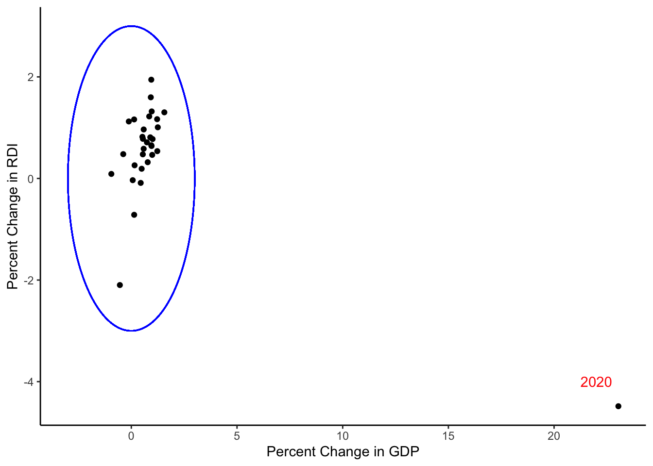
Figure 1: GDP Growth vs RDI Growth: Q7-Q8

Predictive Models

Based on these observations, I built 4 predictive models. Whereas in model (A), the independent variable of interest is RDI growth between Q6 and Q7, in Model (B), I replace that with Q6-Q7 GDP growth. In Model (C), I included unemployment in Q7 as an independent variable because incumbent parties tend to be punished for high unemployment, though the effect may differ based on the party in power (Wright, 2012). (Note that while Wright (2012) suggests that higher unemployment is associated with higher vote shares for Democratic candidates, I was not able to identify such a trend when I ran a regression only for the years in which the incumbent President was a Democrat.) In Model (D), I shed light on the impact of cumulative GDP growth rate (between Q1 and Q7). Comparing Model (C) and Model (D) is important because some suggest that while voters do tend to judge incumbent Presidents based on economic conditions in the election year, they actually want to judge incumbent Presidents based on cumulative records (Healy & Lenz, 2014).

As seen in Table 2, Models (B), (C), and (D) seem promising. Whereas RDI growth did not have a statistically significant impact, GDP growth between Q6 and Q7 had a positive and statistically significant impact on the President’s party’s vote share (Model (B)). In addition to GDP growth, unemployment in Q7 had a negative and statistically significant impact (Model (C)). Interestingly, even after replacing short-term (Q6-Q7) GDP growth rate with cumulative (Q1-Q7) GDP growth rate, I found out that GDP growth rate still had a positive and statistically significant impact. Voters may partially take into account the President’s cumulative records even though they tend to judge the President based on the economic conditions in the election year.

Model Testing and Predictions

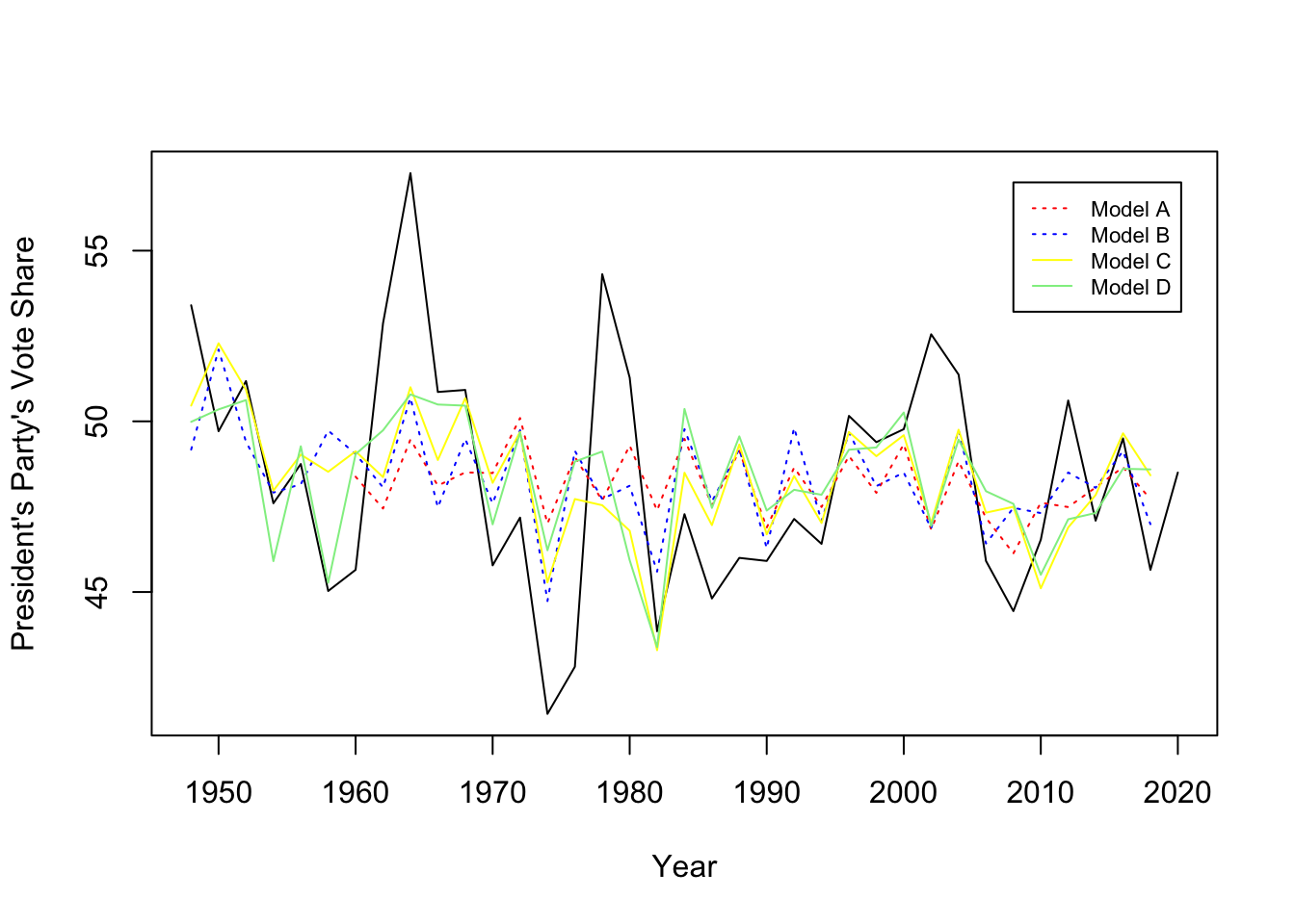
Figure 2: Actual Values vs Predicted Values

By comparing the predicted values based on Models (A) ~ (D) with the actual vote share, we can see that Models (C) and (D) tend to better predict the vote share (Figure 2). Indeed, the adjusted R-squared for Models (C) and (D) are higher than the adjusted R-squared for Models (A) and (B). Also, the root-mean-squared errors are lower for Models (C) and (D) (See Figure 3 for details).

I also conducted out-of-sample model testing to evaluate the models. First, for each of the models, I withheld the observation for the 2018 elections before fitting and observed how well the models predict the vote share in 2018. Here, I observed that model B performed the best (Figure 3, “Leave-One-Out”). Second, I conducted 1000 runs of cross-validation for each of the models, randomly holding out 8 observations in each iteration. As seen in the bottom half of Figure 3, the mean out-of-sample residuals tended to be around -1 to 1. The mean out-of-sample residuals based on Model D seemed to best cluster around 0. Overall, Models (C) and (D) seem to have nearly equivalent predictive power.

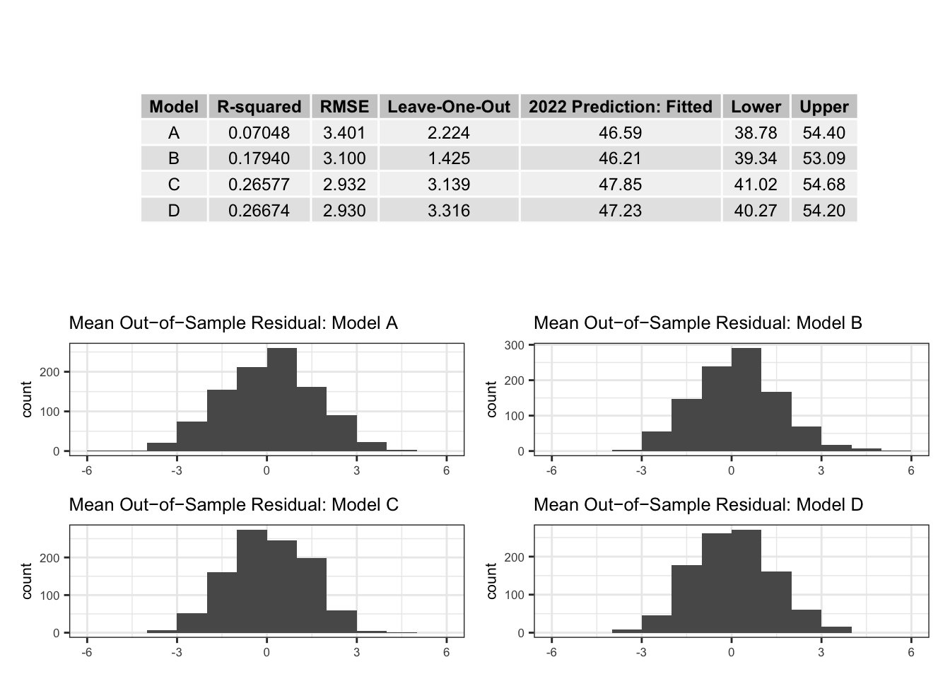
Figure 3: Model Testing & Predictions

Finally, I calculated the predictions for 2022 based on the 4 models. Since the data for Q7 is not available yet, I used the data from Q6 as a substitute. I measured short-term economic growth based on the change between Q6 and Q5 and long-term economic growth based on the change between Q6 and Q1. For all 4 models, the predicted President’s party’s vote share was 46 to 48%. However, since the confidence intervals are wide, it seems that the analysis I did this week is not be enough to accurately predict the outcomes of this election cycle (Figure 3, “2022 Prediction”). Note that there is little difference between Model (C) and Model (D), both in terms of various model evaluation metrics as well as the predicted vote share for 2022. This reinforces my analysis that whether we measure GDP growth using Q6-Q7 records or Q1-Q7 records does not make much difference.

References

Achen, C. H. & Bartels, L. M. (2017). Democracy for realists :why elections do not produce responsive government. Princeton University Press.

Campbell, J. (2018). Introduction: Forecasting the 2018 US Midterm Elections. PS: Political Science & Politics, 51(S1), 1-3. doi:10.1017/S1049096518001592

Healy, A. & Lenz, G. S. (2014). Substituting the End for the Whole: Why Voters Respond Primarily to the Election-Year Economy. American Journal of Political Science, 58(1), 31–47. https://doi.org/10.1111/ajps.12053

Wright, J. R. (2012). Unemployment and the Democratic Electoral Advantage. American Political Science Review, 106(4), 685–702. https://doi.org/10.1017/S0003055412000330